Generalized Plackett-Luce Likelihoods

Robin K. S. Hankin

To cite the hyper2 package in publications, please use Hankin (2017); to cite hyper3 functionality, use Hankin (2024).

The hyper2 package provides functionality to work with extensions of the Bradley-Terry probability model such as Plackett-Luce likelihood including team strengths and reified entities (monsters). The package allows one to use relatively natural R idiom to manipulate such likelihood functions. Here, I present a generalization of hyper2 in which multiple entities are constrained to have identical Bradley-Terry strengths. A new S3 class hyper3, along with associated methods, is motivated and introduced. Three datasets are analysed, each analysis furnishing new insight, and each highlighting different capabilities of the package.

Introduction

The hyper2 package Hankin (2017) furnishes computational support for generalized Plackett-Luce (Plackett 1975) likelihood functions. The preferred interpretation is a race (as in track and field athletics): given six competitors $1-6$, we ascribe to them nonnegative strengths $p_1,\ldots, p_6$; the probability that $i$ beats $j$ is $p_i/(p_i+p_j)$. It is conventional to normalise so that the total strength is unity, and to identify a competitor with his strength. Given an order statistic, say $p_1\succ p_2\succ p_3\succ p_4$, the Plackett-Luce likelihood function would be

$$\begin{equation}\label{PL_like} \frac{p_1}{p_1+p_2+p_3+p_4}\cdot \frac{p_2}{ p_2+p_3+p_4}\cdot \frac{p_3}{ p_3+p_4}\cdot \frac{p_4}{ p_4} \qquad\mbox{Plackett-Luce} \end{equation}$$

Mollica and Tardella (2014) call this a forward ranking process on the grounds that the best (preferred; fastest; chosen) entities are identified in the same sequence as their rank.

Computational support for Bradley-Terry likelihood functions is available in a range of languages. Hunter (2004), for example, presents results in MATLAB [although he works with a nonlinear extension to account for ties]; Allison and Christakis (1994) present related work for ranking statistics in SAS and Maystre (2022) has released a python package for Luce-type choice datasets.

However, the majority of software is written in the R computer language ( Core Team 2023), which includes extensive functionality for working with such likelihood functions: Turner et al. (2020) discuss several implementations from a computational perspective. The BradleyTerry package (Firth 2005) considers pairwise comparisons using glm but cannot deal with ties or player-specific predictors; the BradleyTerry2 package (Turner and Firth 2012) implements a flexible user interface and wider range of models to be fitted to pairwise comparison datasets, specifically simple random effects. The PlackettLuce package (Turner et al. 2020) generalizes this to likelihood functions of the form of the Plackett-Luce equation above, and applies the Poisson transformation of Baker (1994) to express the problem as a log-linear model. The hyper2 package, in contrast, gives a consistent language interface to create and manipulate likelihood functions over the simplex ${S}_n=\left\lbrace\left(p_1,\ldots,p_n\right)\left|p_i\geq 0,\sum p_i=1\right.\right\rbrace$. A further extension in the package generalizes this likelihood function to functions of ${\mathbf p}=(p_1,\ldots,p_n)$ with

$$\begin{equation}\label{hyper2likelihood} \mathcal{L}\left(\mathbf{p}\right)= \prod_{s\in \mathcal{O}}\left({\sum_{i\in s}}p_i\right)^{n_s}\qquad\mbox{Hyperdirichlet likelihood} \end{equation}$$

where $\mathcal{O}$ is a set of observations and $s$ a subset of $\left\{1,2,\ldots,n\right\}$; numbers $n_s$ are integers which may be positive or negative and we usually require $\sum_s n_s=0$. The hyper2 package has the ability to evaluate such likelihood functions at any point in $S_n$, thereby admitting a wide range of non-standard nulls such as order statistics on the $p_i$(Hankin 2017). It becomes possible to analyse a wider range of likelihood functions than standard Plackett-Luce (Turner et al. 2020). For example, results involving incomplete order statistics or teams are tractable. Further, the introduction of reified entities (monsters) allows one to consider draws (Hankin 2010), noncompetitive tactics such as collusion (Hankin 2020), and the phenomenon of team cohesion wherein the team becomes stronger than the sum of its parts (Hankin 2010). Recent versions of the package include experimental functionality cheering() to investigate the relaxing of the assumption of conditional independence of the forward-ranking process.

Here I present a different generalization. Consider a race in which there are six runners 1-6 but we happen to know that three of the runners (1,2,3) are clones of strength $p_a$, two of the runners (4,5) have strength $p_b$, and the final runner (6) is of strength $p_c$. We normalise so $p_a+p_b+p_c=1$. The runners race and the finishing order is:

$$a\succ c\succ b\succ a\succ a \succ b$$

Thus the winner was $a$, second place for $c$, third for $b$, and so on. Alternatively we might say that $a$ came first, fourth, and fifth; $b$ came third and sixth, and $c$ came second. The Plackett-Luce likelihood function for $p_a,p_b,p_c$ would be

$$\begin{equation}\label{plackettluce} \frac{p_a}{3p_a+2p_b+p_c}\cdot \frac{p_c}{2p_a+2p_b+p_c}\cdot \frac{p_b}{2p_a+2p_b }\cdot \frac{p_a}{2p_a+ p_b }\cdot \frac{p_a}{ p_a+ p_b\vphantom{x_{x_{x_{x_{x_{x_{x_{x_{x_{x_{x_{x_{x_{x_{x_{x_{x_{x}}}}}}}}}}}}}}}}}} }\cdot \frac{p_b}{ p_b },\qquad p_a+p_b+p_c=1\\ \mbox{generalized plackett-Luce likelihood} \end{equation}$$

Here I consider such generalized Plackett-Luce likelihood functions, and give an exact analysis of several simple cases. I then show how this class of likelihood functions may be applied to a range of inference problems involving order statistics. Illustrative examples, drawn from Formula 1 motor racing, and track-and-field athletics, are given.

Computational methodology for generalized Plackett-Luce likelihood functions

Existing hyper2 formalism as described by Hankin (2017) cannot represent the Plackett-Luce likelihood equation, because the hyperdirichlet likelihood equation uses sets as the indexing elements, and in this case we need multisets. The declarations

typedef map<string, long double> weightedplayervector;
typedef map<weightedplayervector, long double> hyper3;

show how the map class of the Standard Template Library is used with weightedplayervector objects mapping strings to long doubles (specifically, mapping player names to their multiplicities), and objects of class hyper3 are maps from a weightedplayervector object to long doubles. One advantage of this is efficiency: search, removal, and insertion operations have logarithmic complexity. As an example, the following C++ pseudo code would create a log-likelihood function for the first term in the Plackett-Luce likelihood equation above:

weightedplayervector n,d;
n["a"] = 1; 
d["a"] = 3; 
d["b"] = 2;
d["c"] = 1;

hyper3 L;
L[n] = 1;
L[d] = -1;

Above, we understand n and d to represent numerator and denominator respectively. Object L is an object of class hyper3; it may be evaluated at points in probability space [that is, a vector [a,b,c] of nonnegative values with unit sum] using standard R idiom wrapping C++ back end.

Package implementation

The package includes an S3 class hyper3 for this type of object; extraction and replacement methods use disordR discipline (Hankin 2022). Package idiom for creating such objects uses named vectors:

LL <- hyper3()
LL[c(a = 1)] <- 1
LL[c(a = 3, b = 2, c = 1)] <- -1
LL

## log( (a=1)^1 * (a=3, b=2, c=1)^-1)

Above, we see object LL is a log-likelihood function of the players’ strengths, which may be evaluated at specified points in probability space. A typical use-case would be to assess $H_1\colon p_a=0.9,p_b=0.05,p_c=0.05$ and $H_2\colon p_a=0.01,p_b=0.01,p_c=0.98$, and we may evaluate these hypotheses using generic function loglik():

loglik(c(a = 0.01, b = 0.01, c = 0.98), LL)

## [1] -4.634729

loglik(c(a = 0.90, b = 0.05, c = 0.05), LL)

## [1] -1.15268

Thus we prefer $H_1$ over $H_2$ with about 3.5 units of support, satisfying the standard two units of support criterion (Edwards 1972), and we conclude that our observation [in this case, that one of the three clones of player $a$ beat the $b$ twins and the singleton $c$] furnishes strong support against $H_2$ in favour of $H_1$.

The package includes many helper functions to work with order statistics of this type. Function ordervec2supp3(), for example, can be used to generate a Plackett-Luce log-likelihood function:

(H <- ordervec2supp3(c("a", "c", "b", "a", "a", "b")))

## log( (a=1)^3 * (a=1, b=1)^-1 * (a=2, b=1)^-1 * (a=2, b=2)^-1 * (a=2,
## b=2, c=1)^-1 * (a=3, b=2, c=1)^-1 * (b=1)^1 * (c=1)^1)

(the package gives extensive documentation at ordervec2supp.Rd). We may find a maximum likelihood estimate for the players’ strengths, using generic function maxp(), dispatching to a specialist hyper3 method:

(mH <- maxp(H))

##          a          b          c 
## 0.21324090 0.08724824 0.69951086

(function maxp() uses standard optimization techniques to locate the evaluate; it has access to first derivatives of the log-likelihood and as such has rapid convergence, if its objective function is reasonably smooth).

The package provides a number of statistical tests on likelihood functions, modified from Hankin (2017) to work with hyper3 objects. For example, we may assess the hypothesis that all three players are of equal strength [viz $H_0\colon p_a=p_b=p_c=\frac{1}{3}$]:

equalp.test(H)

## 
##  Constrained support maximization
## 
## data:  H
## null hypothesis: a = b = c
## null estimate:
##         a         b         c 
## 0.3333333 0.3333333 0.3333333 
## (argmax, constrained optimization)
## Support for null:  -6.579251 + K
## 
## alternative hypothesis:  sum p_i=1 
## alternative estimate:
##          a          b          c 
## 0.21324090 0.08724824 0.69951086 
## (argmax, free optimization)
## Support for alternative:  -5.73209 + K
## 
## degrees of freedom: 2
## support difference = 0.8471613
## p-value: 0.42863

showing, perhaps unsurprisingly, that this small dataset is consistent with $H_0$.

Package helper functions

Arithmetic operations are implemented for hyper3 objects in much the same way as for hyper2 objects: independent observations may be combined using the overloaded + operator; an example is given below.

The original motivation for hyper3 was the analysis of Formula 1 motor racing, and the package accordingly includes wrappers for ordervec2supp() such as ordertable2supp3() and attemptstable2supp3() which facilitate the analysis of commonly encountered result formats. Package documentation for order tables is given at ordertable.Rd and an example is given below.

Exact analytical solution for some simple generalized Plackett-Luce likelihood functions

Here I consider some order statistics with nontrivial maximum likelihood Bradley-Terry strengths. The simplest nontrivial case would be three competitors with strengths $a,a,b$ and finishing order $a\succ b\succ a$. The Plackett-Luce likelihood function would be

$$\begin{equation}\label{aba} \frac{a}{2a+b}\cdot\frac{b}{a+b} \end{equation}$$

and in this case we know that $a+b=1$ so this is equal to $\mathcal{L}=\mathcal{L}(a)=\frac{a(1-a)}{1+a}$. The score would be given by

$$\begin{equation}\label{aba_mle} \frac{d\mathcal{L}}{da}=\frac{(1+a)(1-2a)-a(1-a)}{(1+a)^2}= \frac{1-2a-a^2}{(1+a)^2} \end{equation}$$

and this will be zero at $\sqrt{2}-1$; we also note that $d^2\mathcal{L}/da^2=-4(1+a)^{-3}$, manifestly strictly negative for $0\leq a\leq 1$: the root is a maximum.

maxp(ordervec2supp3(c("a", "b", "a")))

##         a         b 
## 0.4142108 0.5857892

Above, we see close agreement with the theoretical value of $(\sqrt{2}-1,2-\sqrt{2})\simeq (0.414,0.586)$. Observe that the maximum likelihood estimate for $a$ is strictly less than 0.5, even though the finishing order is symmetric. Using $\mathcal{L}(a)=\frac{a(1-a)}{1+a}$, we can show that $\log\mathcal{L}(\hat{a})=\log\left(3-2\sqrt{2}\right)\simeq -1.76$, where $\hat{a}=\sqrt{2}-1$ is the maximum likelihood estimate for $a$. Defining $\mathcal{S}=\log\mathcal{L}$ as the support [log-likelihood] we have

$$\begin{equation} \mathcal{S}=\mathcal{S}(a)=\log\left(\frac{a(1-a)}{1+a}\right)-\log\left(3-2\sqrt{2}\right) \end{equation}$$

as a standard support function which has a maximum value of zero when evaluated at $\hat{a}=\sqrt{2}-1$. For example, we can test the null that $a=b=\frac{1}{2}$, the statement that the competitors have equal Bradley-Terry strengths:

a <- 1/2 # null
(S_delta <- log(a * (1 - a)/(1 + a)) - log(3 - 2 * sqrt(2)))

## [1] -0.0290123

Thus the additional support gained in moving from $a=\frac{1}{2}$ to the evaluate of $a=\sqrt{2}-1$ is 0.029, rather small [as might be expected given that we have only one rather uninformative observation, and also given that the maximum likelihood estimate ($\simeq 0.41$) is quite close to the null of $0.5$]. Nevertheless we can follow [Edwards (1972)} and apply Wilks’s theorem for a $p$ value:

pchisq(-2 * S_delta, df = 1, lower.tail = FALSE)

## [1] 0.8096458

The $p$-value is about 0.81, exceeding 0.05; thus we have no strong evidence to reject the null of $a=\frac{1}{2}$. The observation is informative, in the sense that we can find a credible interval for $a$. With an $n$-units of support criterion the analytical solution to $\mathcal{S}(p)=-n$ is given by defining $X=\log(3-2\sqrt{2})-n$ and solving $p(1-p)/(1+p)=X$, or $p_\pm=\left(1-X\pm\sqrt{1+4X+X^2}\right)/2$, the two roots being the lower and upper limits of the credible interval; see the figure below.

a <- seq(from = 0, by = 0.005, to = 1)
S <- function(a){log(a * (1 - a) / ((1 + a) * (3 - 2 * sqrt(2))))}
plot(a, S(a), type = 'b',xlab=expression(p[a]),ylab="support")
abline(h = c(0, -2))
abline(v = c(0.02438102, 0.9524271), col = 'red')
abline(v = sqrt(2) - 1)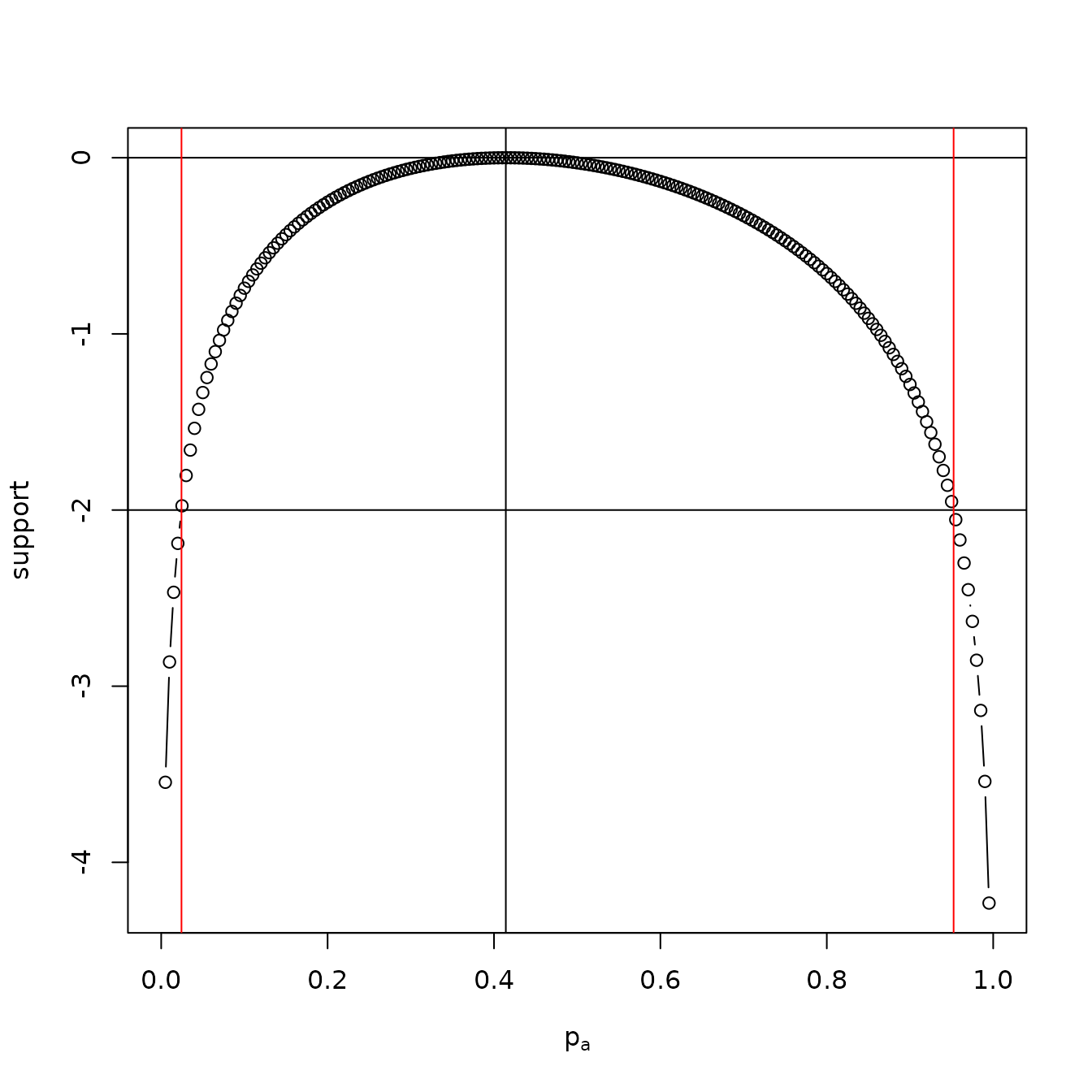

A support function for a>b>a

Fisher information

If we have two clones of $a$ and a singleton $b$, then there are three possible rank statistics: (i), $a\succ a\succ b$ with probability $\frac{2a^2}{1+a}$; (ii), $a\succ b\succ a$, with $\frac{2a(1-a)}{(1+a)}$, (iii), $b\succ a\succ a$ at $\frac{1-a}{1+a}$. Likelihood functions for these order statistics are given in the figure below. It can be shown that the Fisher information for such observations is

$$\begin{equation} \mathcal{I}(a)=2\frac{1+a+a^2}{a(1-a)(1+a)^2} \end{equation}$$

which has a minimum of about $6.21$ at at about $a=0.522$. We can compare this with the Fisher information matrix ${\mathcal I}$, for the case of three distinct runners $a,b,c$, evaluated at its minimum of $p_a=p_b=p_c=\frac{1}{3}$. If we observe the complete order statistic, $\left|{\mathcal I}\right| =\frac{1323}{16}\simeq 82.7$; if we observe just the winner, $\left|{\mathcal I}\right|=27$, and if we observe just the loser we have $\left|{\mathcal I}\right|=\frac{16875}{256}\simeq 65.9$. A brief discussion is given at inst/fisher_inf_PL3.Rmd.

f_aab <- function(a){a^2 / (1 + a)}
f_aba <- function(a){a * (1 - a) / (1 + a)}
f_baa <- function(a){(1 - a) / (1 + a)}
p <- function(f, ...){
  a <- seq(from = 0, by = 0.005, to = 1)
  points(a, f(a) / max(f(a)), ...)
  }
plot(0:1, 0:1, xlab = expression(p[a]), ylab = "Likelihood", type = "n")
p(f_aab, type = "l", col = "black")
p(f_aba, type = "l", col = "red")
p(f_baa, type = "l", col = "blue")
text(0.8,0.8,"AAB")
text(0.8,0.4,"ABA",col="red")
text(0.8,0.05,"BAA",col="blue")
abline(h = exp(-2), lty = 2)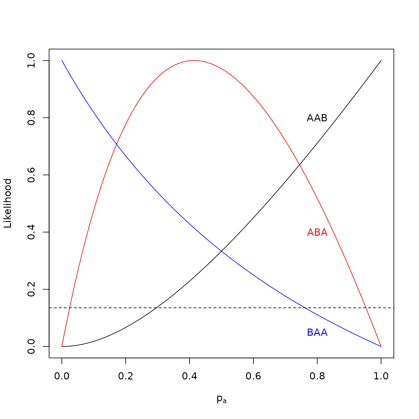

Support functions for observations a>a>b, a>b>a and b>a>a. Horizontal dotted line represents two units of support

Nonfinishers

If we allow non-finishers—that is, a subset of competitors who are beaten by all the ranked competitors ((Turner et al. 2020) call this a top $n$ ranking), there is another nontrivial order statistic, viz $a\succ b\succ\left\lbrace a,b\right\rbrace$ [thus one of the two $a$’s won, one of the $b$’s came second, and one of each of $a$ and $b$ failed to finish]. Now

$$\begin{equation} \mathcal{L}(a)= \frac{a}{2a+2b}\cdot \frac{b}{ a+2b}\propto\frac{a(1-a)}{2-a} \end{equation}$$

(see how the likelihood function is actually simpler than for the complete order statistic). The evaluate would be $2-\sqrt{2}\simeq 0.586$:

maxp(ordervec2supp3(c("a", "b"), nonfinishers=c("a", "b")))

##         a         b 
## 0.5857892 0.4142108

The Fisher information for such observations has a minimum of $\frac{68}{9}\simeq 7.56$ at $a=\frac{1}{2}$. An inference problem for a dataset including nonfinishers will be given below.

An alternative to the Mann-Whitney test using generalized Plackett-Luce likelihood

The ideas presented above can easily be extended to arbitrarily large numbers of competitors, although the analytical expressions tend to be intractable and numerical methods must be used. All results and datasets presented here are maintained under version control and available at https://github.com/RobinHankin/hyper2. Given an order statistic of the type considered above, the Mann-Whitney-Wilcoxon test (Mann and Whitney 1947, wilcoxon1945) assesses a null of identity of underlying distributions (Ahmad 1996). Consider the chorioamnion dataset (Hollander, Wolfe, and Chicken 2013), used in wilcox.test.Rd:

x <- c(0.80, 0.83, 1.89, 1.04, 1.45, 1.38, 1.91, 1.64, 0.73, 1.46)
y <- c(1.15, 0.88, 0.90, 0.74, 1.21)

Here we see a measure of permeability of the human placenta at term (x) and between 3 and 6 months’ gestational age (y). The order statistic is straightforward to calculate:

names(x) <- rep("x", length(x))
names(y) <- rep("y", length(y))
(os <- names(sort(c(x, y))))

##  [1] "x" "y" "x" "x" "y" "y" "x" "y" "y" "x" "x" "x" "x" "x" "x"

Then object os is converted to a hyper3 object, again with ordervec2supp3(), which may be assessed using the Method of Support:

Hxy <- ordervec2supp3(os)
equalp.test(Hxy)

## 
##  Constrained support maximization
## 
## data:  Hxy
## null hypothesis: x = y
## null estimate:
##   x   y 
## 0.5 0.5 
## (argmax, constrained optimization)
## Support for null:  -27.89927 + K
## 
## alternative hypothesis:  sum p_i=1 
## alternative estimate:
##         x         y 
## 0.2401539 0.7598461 
## (argmax, free optimization)
## Support for alternative:  -26.48443 + K
## 
## degrees of freedom: 1
## support difference = 1.414837
## p-value: 0.09253716

Above, we use generic function equalp.test() to test the null that the permeability of the two groups both have Bradley-Terry strength of $0.5$. We see a $p$ value of about 0.09; compare 0.25 from wilcox.test(). However, observe that the hyper3 likelihood approach gives more information than Wilcoxon’s analysis: Firstly, we see that the maximum likelihood estimate for the Bradley-Terry strength of x is about 0.24, considerably less than the null of 0.5; further, we may plot a support curve for this dataset, given in the figure below.

a <- seq(from = 0.02, to = 0.8, len = 40)
L <- sapply(a, function(p){loglik(p, Hxy)})
plot(a, L - max(L), type = 'b',xlab=expression(p[a]),ylab="likelihood")
abline(h = c(0, -2))
abline(v = c(0.24))
abline(v=c(0.5), lty=2)

A support function for the Bradley-Terry strength of permeability at term. The evaluate of 0.24 is shown; and the two-units-of support credible interval, which does not exclude the null of strength 0.5 (dotted line), is also shown

A generalization of the Mann-Whitney test using generalized Plackett-Luce likelihood

The ideas presented above may be extended to more than two types of competitors. Consider the following table, drawn from the men’s javelin, 2020 Olympics:

javelin_table

##           throw1 throw2 throw3 throw4 throw5 throw6
## Chopra     87.03  87.58  76.79      X      X  84.24
## Vadlejch   83.98      X      X  82.86  86.67      X
## Vesely     79.73  80.30  85.44      X  84.98      X
## Weber      85.30  77.90  78.00  83.10  85.15  75.72
## Nadeem     82.40      X  84.62  82.91  81.98      X
## Katkavets  82.49  81.03  83.71  79.24      X      X
## Mardare    81.16  81.73  82.84  81.90  83.30  81.09
## Etelatalo  78.43  76.59  83.28  79.20  79.99  83.05

Thus Chopra threw 87.03m on his first throw, 87.58m on his second, and so on. No-throws, ignored here, are indicated with an X. We may convert this to a named vector with elements being the throw distances, and names being the competitors, using attemptstable2supp3():

javelin_vector <- attemptstable2supp3(javelin_table,
       decreasing = TRUE, give.supp = FALSE)
options(width = 60)
javelin_vector

##    Chopra    Chopra  Vadlejch    Vesely     Weber     Weber 
##     87.58     87.03     86.67     85.44     85.30     85.15 
##    Vesely    Nadeem    Chopra  Vadlejch Katkavets   Mardare 
##     84.98     84.62     84.24     83.98     83.71     83.30 
## Etelatalo     Weber Etelatalo    Nadeem  Vadlejch   Mardare 
##     83.28     83.10     83.05     82.91     82.86     82.84 
## Katkavets    Nadeem    Nadeem   Mardare   Mardare   Mardare 
##     82.49     82.40     81.98     81.90     81.73     81.16 
##   Mardare Katkavets    Vesely Etelatalo    Vesely Katkavets 
##     81.09     81.03     80.30     79.99     79.73     79.24 
## Etelatalo Etelatalo     Weber     Weber    Chopra Etelatalo 
##     79.20     78.43     78.00     77.90     76.79     76.59 
##     Weber  Vadlejch    Nadeem  Vadlejch    Chopra    Vesely 
##     75.72        NA        NA        NA        NA        NA 
##    Chopra Katkavets  Vadlejch    Vesely    Nadeem Katkavets 
##        NA        NA        NA        NA        NA        NA

Above we see that Chopra threw the longest and second-longest throws of 87.58m and 87.03 respectively; Vadlejch threw the third-longest throw of 86.67m, and so on (NA entries correspond to no-throws.) The attempts table may be converted to a hyper3 object, again using function attemptstable2supp3() but this time passing give.supp=TRUE:

javelin <- ordervec2supp3(v = names(javelin_vector)[!is.na(javelin_vector)])

Above, object javelin is a hyper3 likelihood function, so one has access to the standard likelihood-based methods, such as finding and displaying the maximum likelihood estimate, shown in the figure below.

(mj <- maxp(javelin))

##    Chopra Etelatalo Katkavets   Mardare    Nadeem  Vadlejch 
##    0.0930    0.0482    0.0929    0.1173    0.1730    0.3206 
##    Vesely     Weber 
##    0.1140    0.0409

dotchart(mj, pch = 16,xlab="Estimated Bradley-Terry strength")

Maximum likelihood estimate for javelin throwers’ Bradley-Terry strengths

From this, we see that Vadlejch has the highest estimated Bradley-Terry strength, but further analysis with equalp.test() reveals that there is no strong evidence in the dataset to reject the hypothesis of equal competitive strength ($p=0.26$), or that Vadlejch has a strength higher than the null value of $\frac{1}{8}$ ($p=0.1$).

A particularly attractive feature of this analysis is that the Bradley-Terry strengths have direct operational significance: If two competitors, say Vadlejch and Vesely, were to throw a javelin, then we would estimate the probability that Vadlejch would throw further than Vesely at $\displaystyle p_{\mbox{Vad}}/\left(p_{\mbox{Vad}} + p_{\mbox{Ves}}\right)\simeq 0.74$. Indeed, from a training or selection perspective we might follow Hankin (2017) and observe that log-contrasts (O’Hagan and Forster 2004) appear to have approximately Gaussian likelihood functions for observations of the type considered here. Profile log-likelihood curves for log-contrasts are easily produced by the package, below.

Profile likelihood for log-contrast as per the text. Null indicated with a dotted line, and two-units-of-support limit indicated with horizontal lines; thus the null is not rejected

We see that the credible range for $\log\left(p_{\mbox{Vad}}/ p_{\mbox{Ves}}\right)$ includes zero and we have no strong evidence for these athletes having different (Bradley-Terry) strengths.

Formula 1 motor racing: The Constructors’ Championship

Formula 1 motor racing is an important and prestigious motor sport (Codling 2017, jenkins2010). In Formula 1 Grand Prix, the constructors’ championship takes place between manufacturers of racing cars (compare the drivers’ championship, which is between drivers). In this analysis, the constructor is the object of inference. Each constructor typically fields two cars, each of which separately accumulates ranking-based points at each venue. Here we use a generalized Plackett-Luce model to assess the constructors’ performance. The following table, included in the hyper2 package as a dataset, shows rankings for the first 9 venues of the 2021 season:

constructor_2021_table[, 1:9]

##    Constructor BHR EMI POR ESP  MON AZE FRA STY
## 1         Merc   1   2   1   1    7  12   2   2
## 2         Merc   3 Ret   3   3  Ret  15   4   3
## 3         RBRH   2   1   2   2    1   1   1   1
## 4         RBRH   5  11   4   5    4  18   3   4
## 5      Ferrari   6   4   6   4    2   4  11   6
## 6      Ferrari   8   5  11   7 DNSP   8  16   7
## 7           MM   4   3   5   6    3   5   5   5
## 8           MM   7   6   9   8   12   9   6  13
## 9           AR  13   9   7   9    9   6   8   9
## 10          AR Ret  10   8  17   13 Ret  14  14
## 11         ATH   9   7  10  10    6   3   7  10
## 12         ATH  17  12  15 Ret   16   7  13 Ret
## 13         AMM  10   8  13  11    5   2   9   8
## 14         AMM  15  15  14  13    8 Ret  10  12
## 15          WM  14 Ret  16  14   14  16  12  17
## 16          WM  18 Ret  18  16   15  17  18 Ret
## 17        ARRF  11  13  12  12   10  10  15  11
## 18        ARRF  12  14 Ret  15   11  11  17  15
## 19          HF  16  16  17  18   17  13  19  16
## 20          HF Ret  17  19  19   18  14  20  18

Above, we see that Mercedes (“Merc”) came first and third at Bahrain (BHR); and came second and retired at Emilia Romagna (EMI); full details of the notation and conventions are given in the package at constructor.Rd. The identity of the driver is viewed as inadmissible information and indeed may change during a season. Alternatively, we may regard the driver and the constructor as a joint entity, with the constructor’s ability to attract and retain a skilled driver being part of the object of inference. The associated generalized Plackett-Luce hyper3 object is easily constructed using package idiom, in this case ordertable2supp3(), and we may use this to assess the Plackett-Luce strengths of the constructors:

const2020 <- ordertable2supp3(constructor_2020_table)
const2021 <- ordertable2supp3(constructor_2021_table)
options(digits=4)

maxp(const2020)
##    ARRF     ATH Ferrari      HF    Merc      MR       R 
## 0.04530 0.06807 0.06063 0.02623 0.37783 0.10026 0.09767 
##    RBRH  RPBWTM      WM 
## 0.12072 0.08055 0.02273

maxp(const2021)
##     AMM      AR    ARRF     ATH Ferrari      HF    Merc 
## 0.05942 0.07543 0.06238 0.05611 0.16939 0.02023 0.19395 
##      MM    RBRH      WM 
## 0.14126 0.18334 0.03848

Above, we see the strength of Mercedes falling from about 0.38 in 2020 to less than 0.20 in 2021 and it is natural to wonder whether this can be ascribed to random variation. Observe that testing such a hypothesis is complicated by the fact that constructors field multiple cars, and also that constructors come and go, with two 2020 teams dropping out between years and two joining. We may test this statistically by defining a combined likelihood function for both years, keeping track of the year:

H <- (
      psubs(constructor_2020, "Merc", "Merc2020") +
      psubs(constructor_2021, "Merc", "Merc2021")
     )

Above, we use generic function psubs() to change the name of Mercedes from Merc to Merc2020 and Merc2021 respectively. Note the use of + to represent addition of log-likelihoods, corresponding to the assumption of conditional independence of results. The null would be simply that the strengths of Merc2020 and of Merc2021 are identical. Package idiom would be to use generic function samep.test():

options(digits = 4)
samep.test(H, c("Merc2020", "Merc2021"))

## 
##  Constrained support maximization
## 
## data:  H
## null hypothesis: Merc2020 = Merc2021
## null estimate:
##      AMM       AR     ARRF      ATH  Ferrari       HF 
##  0.04239  0.05413  0.04677  0.04374  0.07568  0.02323 
## Merc2020 Merc2021       MM       MR        R     RBRH 
##  0.13903  0.13903  0.09016  0.07944  0.07475  0.10024 
##   RPBWTM       WM 
##  0.06235  0.02905 
## (argmax, constrained optimization)
## Support for null:  -1189 + K
## 
## alternative hypothesis:  sum p_i=1 
## alternative estimate:
##      AMM       AR     ARRF      ATH  Ferrari       HF 
##  0.03766  0.04824  0.04333  0.04060  0.07036  0.02132 
## Merc2020 Merc2021       MM       MR        R     RBRH 
##  0.23135  0.09216  0.07893  0.07973  0.07455  0.09322 
##   RPBWTM       WM 
##  0.06177  0.02679 
## (argmax, free optimization)
## Support for alternative:  -1184 + K
## 
## degrees of freedom: 1
## support difference = 4.722
## p-value: 0.002119

Above, we see strong evidence for a real decrease in the strength of the Mercedes team from 2020 to 2021, with $p=0.002$.

Conclusions and further work

Plackett-Luce likelihood functions for rank datasets have been generalized to impose identity of Bradley-Terry strengths for certain groups; the preferred interpretation is a running race in which the competitors are split into equivalence classes of clones. Implementing this in R is accomplished via a C++ back-end making use of the STL “map” class which offers efficiency advantages, especially for large objects.

New likelihood functions for simple cases with three or four competitors were presented, and extending to larger numbers furnishes a generalization of the Mann-Whitney-Wilcoxon test that offers a specific alternative (Bradley-Terry strength) with a clear operational definition. Further generalizations allow the analysis of more than two groups, here applied to Olympic javelin throw distances. Generalized Plackett-Luce likelihood functions were used to assess the Grand Prix constructors’ championship and a reasonable null. Specifically, the hypothesis that the strength of the Mercedes team remained unchanged between 2020 and 2021 was tested and rejected.

Draws are not considered in the present work but in principle may be accommodated, either using likelihoods comprising sums of Plackett-Luce probabilities (Hankin 2017); or the introduction of a reified draw entity (Hankin 2010).

Further work might include a systematic comparison between hyper3 approach and the Mann-Whitney-Wilcoxon test, including the characterisation of the power function of both tests. The package could easily be extended to allow non-integer multiplicities, which might prove useful in the context of reified Bradley Terry techniques (Hankin 2020).

References

Ahmad, I. A. 1996. “A Class of Mann-Whitney-Wilcoxon Type Statistics.” The American Statistician 50 (4): 324–27.

Allison, P. D., and N. A. Christakis. 1994. “Logit Models for Sets of Ranked Items.” Sociological Methodology 24: 199–228.

Baker, S. G. 1994. “The Multinomial-Poisson Transformation.” The Statistician 43 (4): 495–504.

Codling, S. 2017. Speed Read F1. Motorbooks.

Core Team. 2023. : A Language and Environment for Statistical Computing. Vienna, Austria: Foundation for Statistical Computing. https://www.R-project.org/.

Edwards, A. W. F. 1972. Likelihood. John Hopkins University Press.

Firth, David. 2005. “Bradley-Terry Models in R.” Journal of Statistical Software 12 (1).

Hankin, R. K. S. 2010. “A Generalization of the Dirichlet Distribution.” Journal of Statistical Software 33 (11): 1–18. https://doi.org/10.18637/jss.v033.i11.

———. 2017. “Partial Rank Data with the hyper2 Package: Likelihood Functions for Generalized Bradley-Terry Models.” The R Journal 9 (2): 429–39.

———. 2020. “A Generalization of the Bradley-Terry Model for Draws in Chess with an Application to Collusion.” Journal of Economic Behavior and Organization 180: 325–33.

———. 2022. : Non-Ordered Vectors. https://github.com/RobinHankin/disordR.

———. 2024. “Generalized Plackett-Luce Likelihoods.” Journal of Statistical Software 109 (8). https://doi.org/10.18637/jss.v109.i08.

Hollander, M., D. A. Wolfe, and E. Chicken. 2013. Nonparametric Statistical Methods. 3rd ed. John Wiley. https://doi.org/https://doi.org/10.1002/9781119196037.

Hunter, D. R. 2004. “MM Algorithms for Generalized Bradley-Terry Models.” The Annals of Statistics 32 (1): 384–406.

Mann, H. B., and D. R. Whitney. 1947. “On a Test of Whether One of Two Random Variables Is Stochastically Larger Than the Other.” Ann. Math. Statist. 18 (1): 50–60. https://doi.org/https://doi.org/10.1214/aoms/1177730491.

Maystre, L. 2022. : Inference Algorithms for Models Based on Luce’s Choice Axiom. https://github.com/lucasmaystre/choix.

Mollica, C., and L. Tardella. 2014. “Epitope Profiling via Mixture Modeling of Ranked Data.” Statistics in Medicine 33: 3738–58.

O’Hagan, A., and J. Forster. 2004. Kendall’s Advanced Theory of Statistics, Volume 2B: Bayesian Inference. 2nd ed. John Wiley & Sons. https://doi.org/https://doi.org/10.1111/j.1467-985x.2004.00347_15.x.

Plackett, R. L. 1975. “The Analysis of Permutations.” Applied Statistics 24: 193–202.

Turner, H. L., and David Firth. 2012. “Bradley-Terry Models in : The Package.” Journal of Statistical Software 48 (9): 1–21. https://doi.org/10.18637/jss.v048.i09.

Turner, H. L., Jacob van Etten, David Firth, and Ioannis Kosmidis. 2020. “Modelling Rankings in : The Package.” Computational Statistics 35: 1027–57. https://doi.org/10.1007/s00180-020-00959-3.