Jacobi form of the elliptic functions

Jacobian elliptic functions

ss(u,m, ...)
sc(u,m, ...)
sn(u,m, ...)
sd(u,m, ...)
cs(u,m, ...)
cc(u,m, ...)
cn(u,m, ...)
cd(u,m, ...)
ns(u,m, ...)
nc(u,m, ...)
nn(u,m, ...)
nd(u,m, ...)
ds(u,m, ...)
dc(u,m, ...)
dn(u,m, ...)
dd(u,m, ...)

Arguments

u

Complex argument

m

Parameter

...

Extra arguments, such as maxiter, passed to theta.?()

Details

All sixteen Jacobi elliptic functions.

References

M. Abramowitz and I. A. Stegun 1965. Handbook of mathematical functions. New York: Dover

Author

Robin K. S. Hankin

See also

theta

Examples

#Example 1, p579:
nc(1.9965,m=0.64)
#> [1] -1392.111
# (some problem here)

# Example 2, p579:
dn(0.20,0.19)
#> [1] 0.9962527

# Example 3, p579:
dn(0.2,0.81)
#> [1] 0.984056

# Example 4, p580:
cn(0.2,0.81)
#> [1] 0.9802785

# Example 5, p580:
dc(0.672,0.36)
#> [1] 1.174019

# Example 6, p580:
Theta(0.6,m=0.36)
#> [1] 0.9735688

# Example 7, p581:
cs(0.53601,0.09)
#> [1] 1.691832

# Example 8, p581:
sn(0.61802,0.5)
#> [1] 0.5645758

#Example 9, p581:
sn(0.61802,m=0.5)
#> [1] 0.5645758

#Example 11, p581:
cs(0.99391,m=0.5)
#> [1] 0.7499963
# (should be 0.75 exactly)

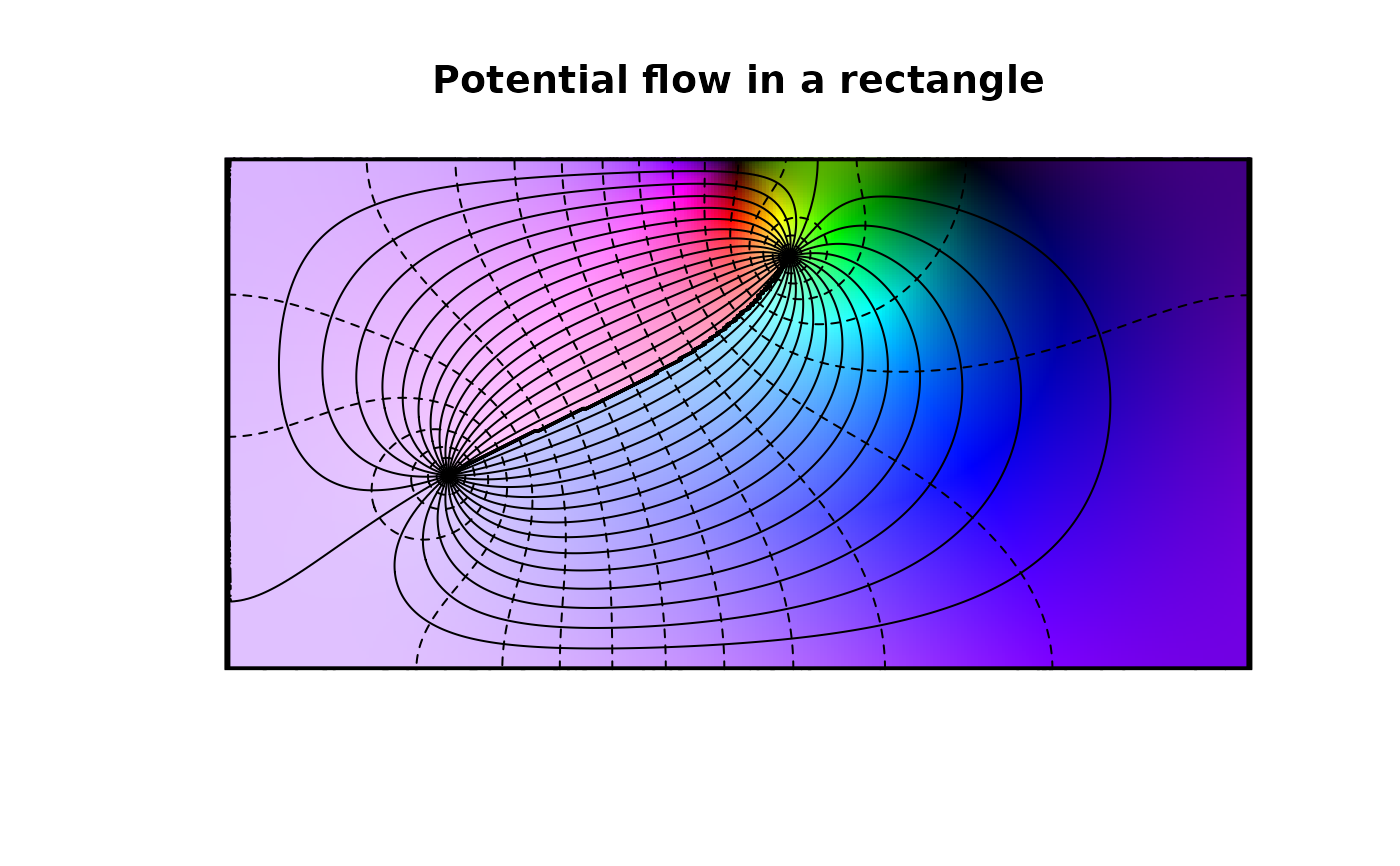
#and now a pretty picture:

n <- 300
K <- K.fun(1/2)
f <- function(z){1i*log((z-1.7+3i)*(z-1.7-3i)/(z+1-0.3i)/(z+1+0.3i))}
# f <- function(z){log((z-1.7+3i)/(z+1.7+3i)*(z+1-0.3i)/(z-1-0.3i))}
x <- seq(from=-K,to=K,len=n)
y <- seq(from=0,to=K,len=n)
z <- outer(x,1i*y,"+")

view(x, y, f(sn(z,m=1/2)), nlevels=44, imag.contour=TRUE,
     real.cont=TRUE, code=1, drawlabels=FALSE,
     main="Potential flow in a rectangle",axes=FALSE,xlab="",ylab="")
rect(-K,0,K,K,lwd=3)