Visualization of complex functions

Visualization of complex functions using colour maps and contours

view(x, y, z, scheme = 0, real.contour = TRUE, imag.contour = real.contour,
default = 0, col="black", r0=1, power=1, show.scheme=FALSE, ...)

Arguments

x,y

Vectors showing real and imaginary components of complex plane; same functionality as arguments to image()

z

Matrix of complex values to be visualized

scheme

Visualization scheme to be used. A numeric value is interpreted as one of the (numbered) provided schemes; see source code for details, as I add new schemes from time to time and the code would in any case dominate anything written here.

A default of zero corresponds to Thaller (1998): see references. For no colour (ie a white background), set scheme to a negative number.

If scheme does not correspond to a built-in function, the switch() statement “drops through” and provides a white background (use this to show just real or imaginary contours; a value of \(-1\) will always give this behaviour)

If not numeric, scheme is interpreted as a function that produces a colour; see examples section below. See details section for some tools that make writing such functions easier

real.contour,imag.contour

Boolean with default TRUE meaning to draw contours of constant \(Re(z)\) (resp: \(Im(z)\)) and FALSE meaning not to draw them

default

Complex value to be assumed for colouration, if z takes NA or infinite values; defaults to zero. Set to NA for no substitution (ie plot z “as is”); usually a bad idea

col

Colour (sent to contour())

r0

If scheme=0, radius of Riemann sphere as used by Thaller

power

Defines a slight generalization of Thaller's scheme. Use high values to emphasize areas of high modulus (white) and low modulus (black); use low values to emphasize the argument over the whole of the function's domain.

This argument is also applied to some of the other schemes where it makes sense

show.scheme

Boolean, with default FALSE meaning to perform as advertized and visualize a complex function; and TRUE meaning to return the function corresponding to the value of argument scheme

...

Extra arguments passed to image() and contour()

Details

The examples given for different values of scheme are intended as examples only: the user is encouraged to experiment by passing homemade colour schemes (and indeed to pass such schemes to the author).

Scheme 0 implements the ideas of Thaller: the complex plane is mapped to the Riemann sphere, which is coded with the North pole white (indicating a pole) and the South Pole black (indicating a zero). The equator (that is, complex numbers of modulus r0) maps to colours of maximal saturation.

Function view() includes several tools that simplify the creation of suitable functions for passing to scheme.

These include:

breakup():

Breaks up a continuous map: function(x){ifelse(x>1/2,3/2-x,1/2-x)}

g():

maps positive real to \([0,1]\): function(x){0.5+atan(x)/pi}

scale():

scales range to \([0,1]\): function(x){(x-min(x))/(max(x)-min(x))}

wrap():

wraps phase to \([0,1]\): function(x){1/2+x/(2*pi)}

Author

Robin K. S. Hankin

Note

Additional ellipsis arguments are given to both image() and contour() (typically, nlevels). The resulting warning() from one or other function is suppressed by suppressWarnings().

References

B. Thaller 1998. Visualization of complex functions, The Mathematica Journal, 7(2):163–180

Examples

n <- 100
x <- seq(from=-4,to=4,len=n)
y <- x
z <- outer(x,1i*y,"+")
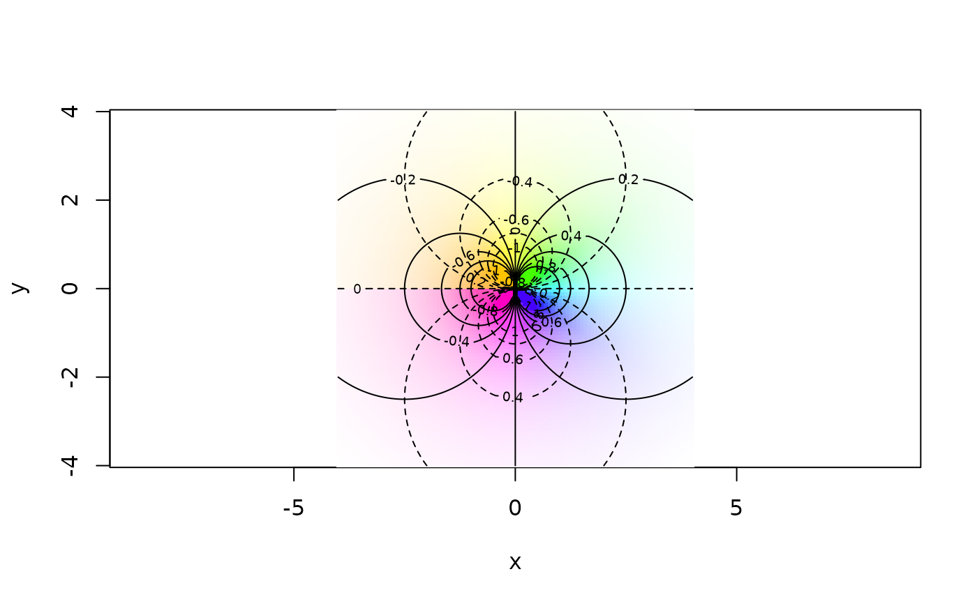
view(x,y,limit(1/z),scheme=2)

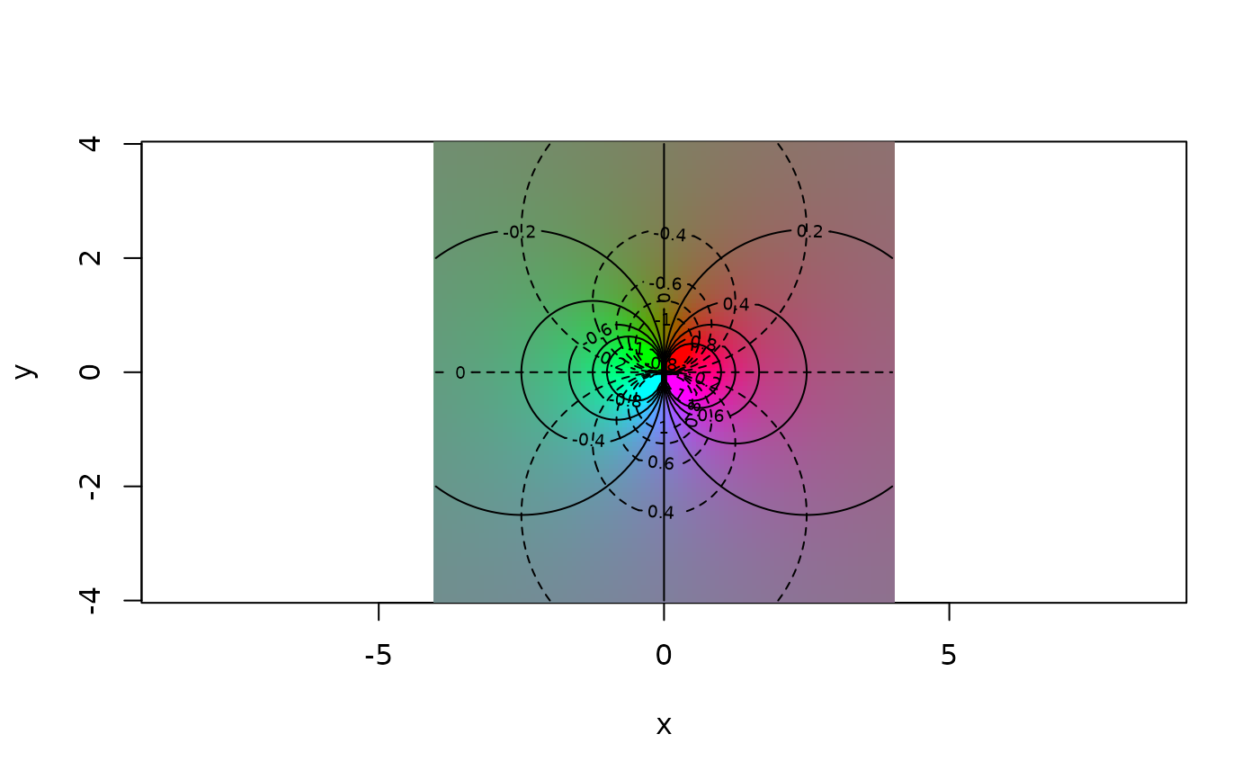
view(x,y,limit(1/z),scheme=18)



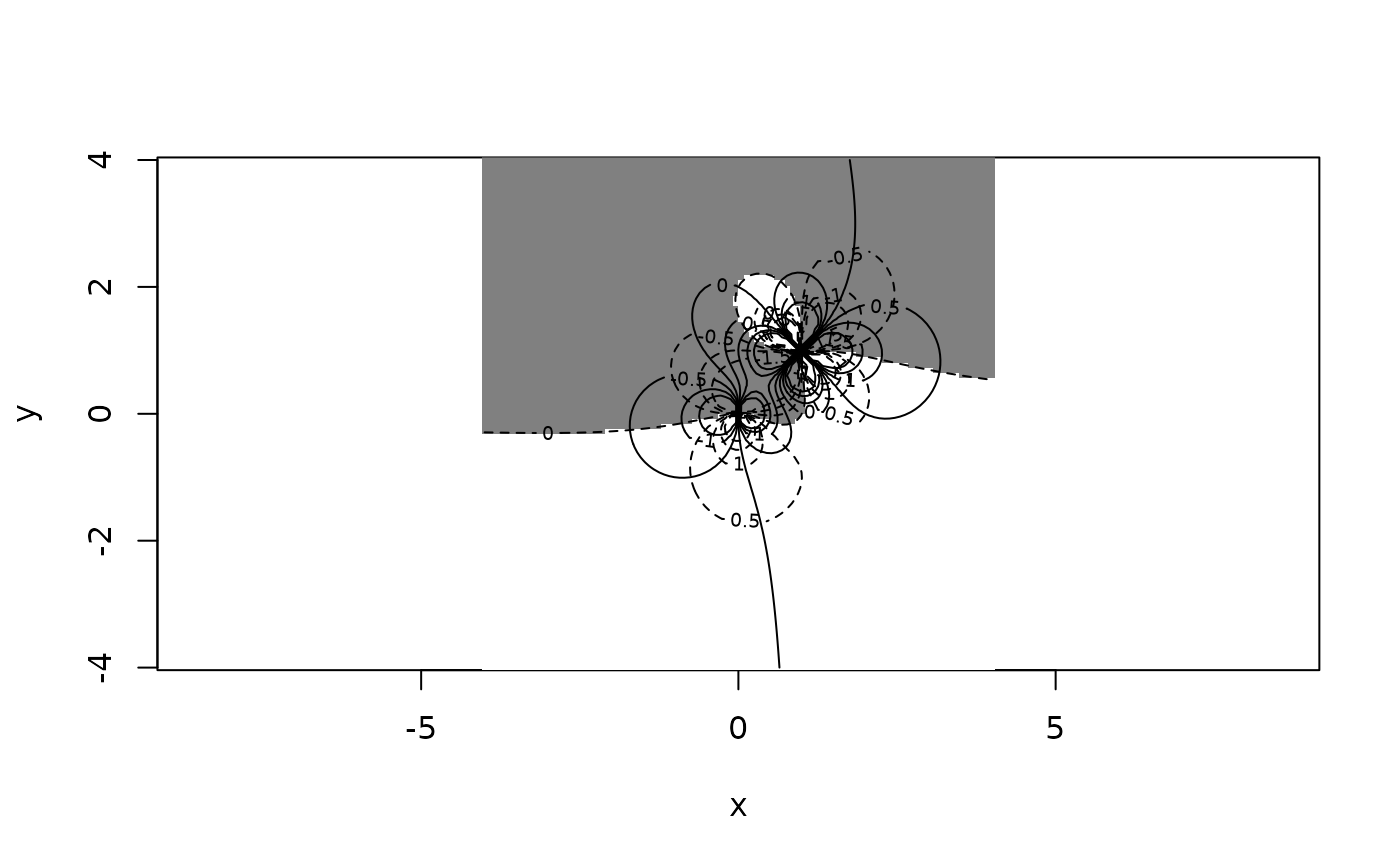
view(x,y,limit(1/z+1/(z-1-1i)^2),scheme=5)

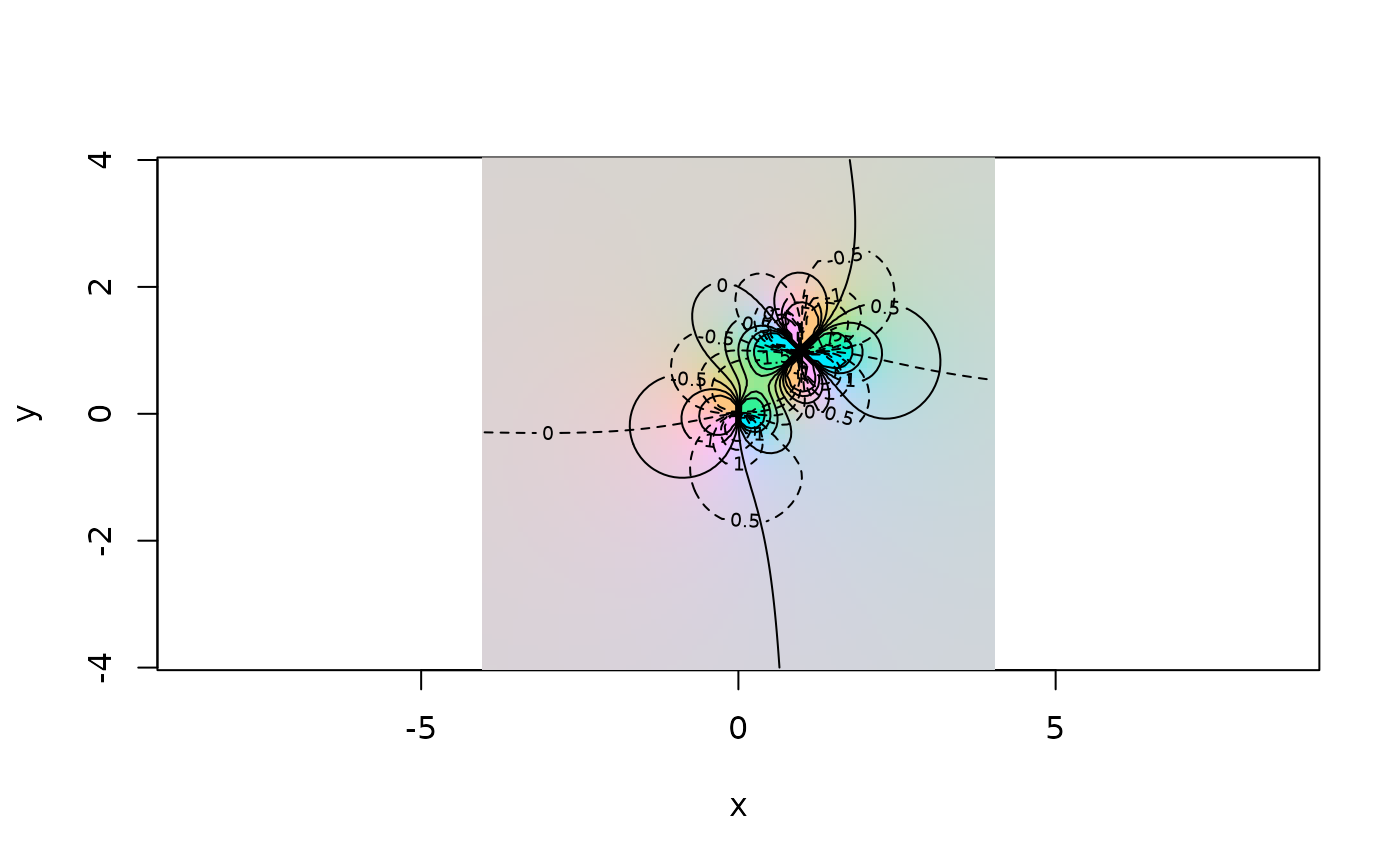
view(x,y,limit(1/z+1/(z-1-1i)^2),scheme=17)


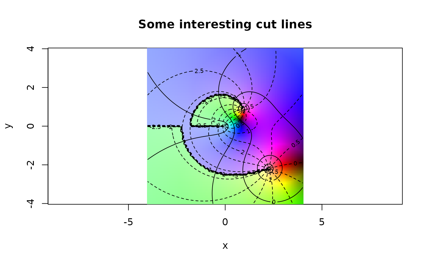
view(x,y,log(0.4+0.7i+log(z/2)^2),main="Some interesting cut lines")



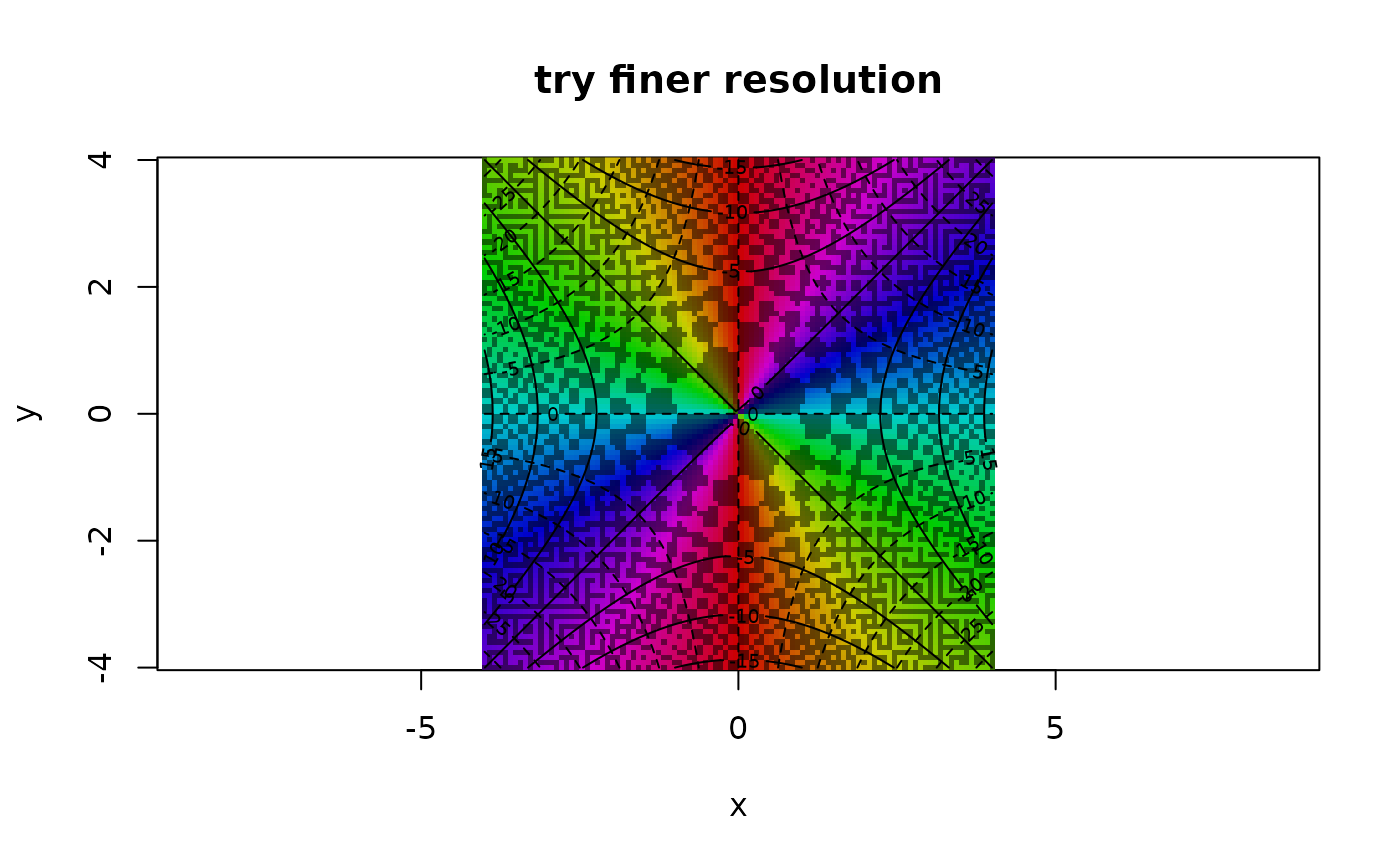
view(x,y,z^2,scheme=15,main="try finer resolution")

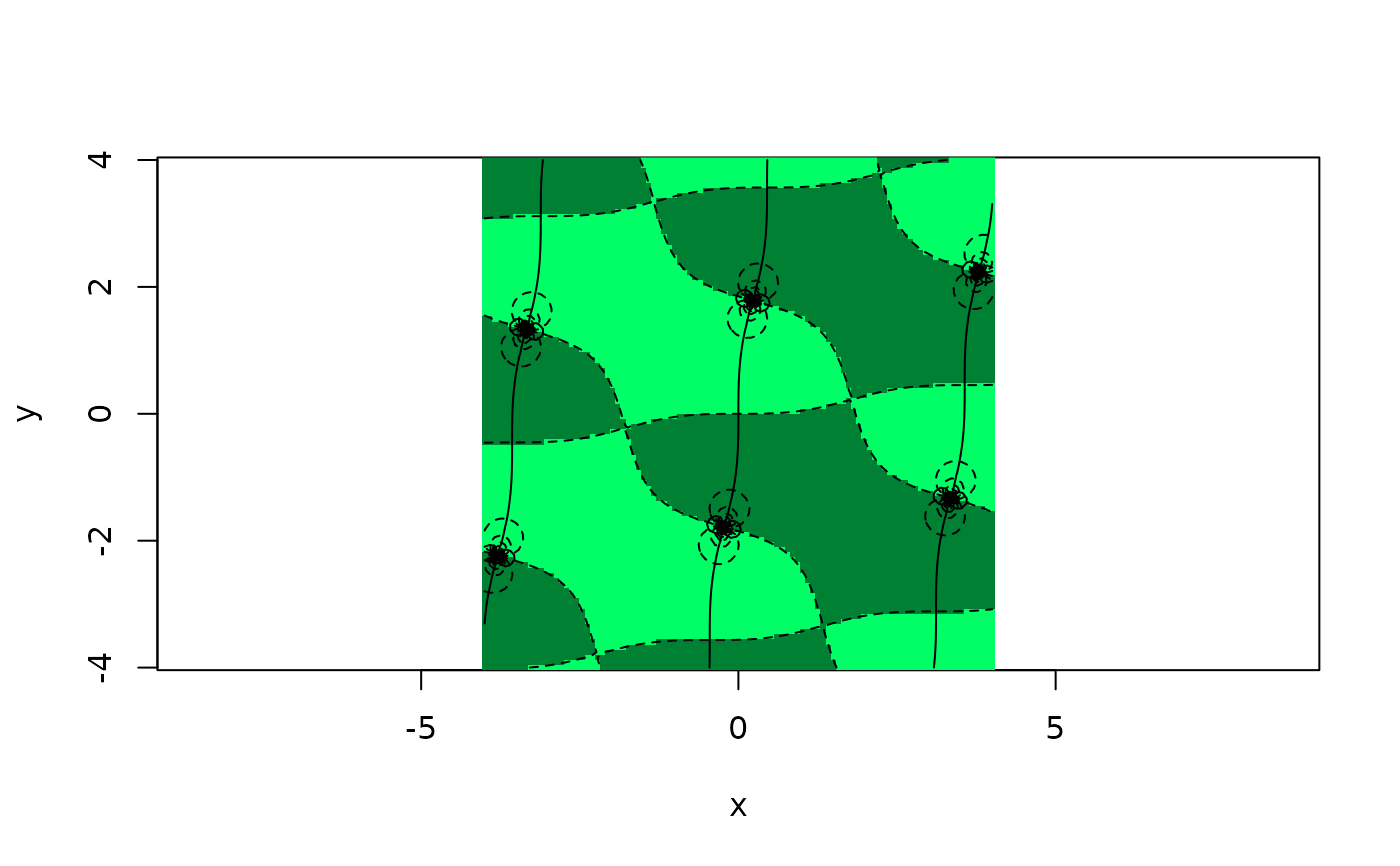
view(x,y,sn(z,m=1/2+0.3i),scheme=6,nlevels=33,drawlabels=FALSE)


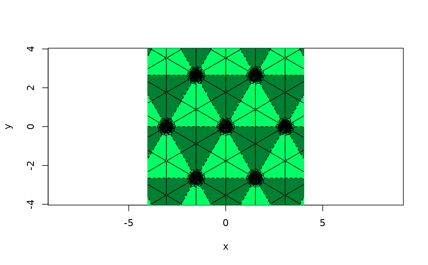
view(x,y,limit(P(z,c(1+2.1i,1.3-3.2i))),scheme=2,nlevels=6,drawlabels=FALSE)

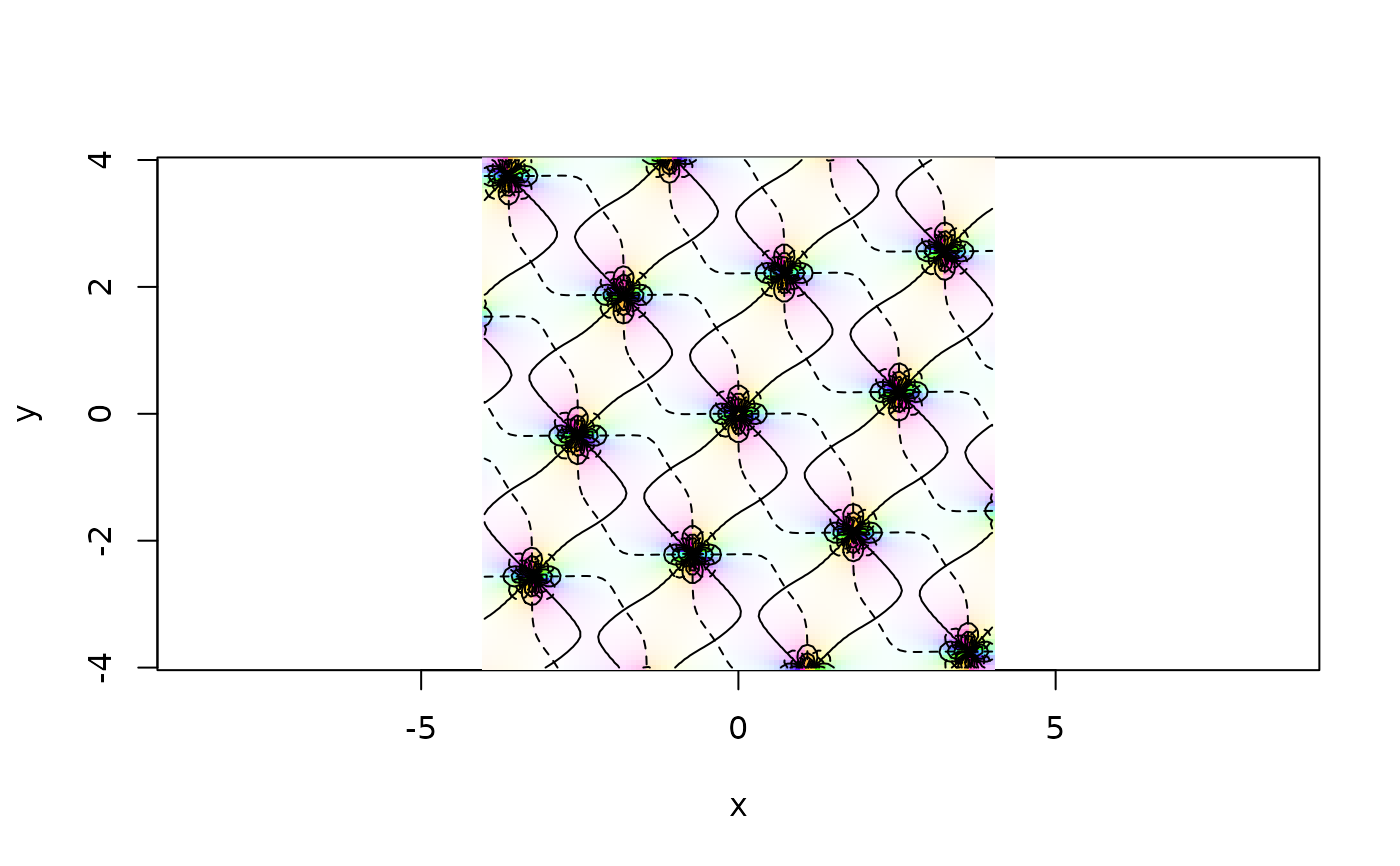view(x,y,limit(Pdash(z,c(0,1))),scheme=6,nlevels=7,drawlabels=FALSE)

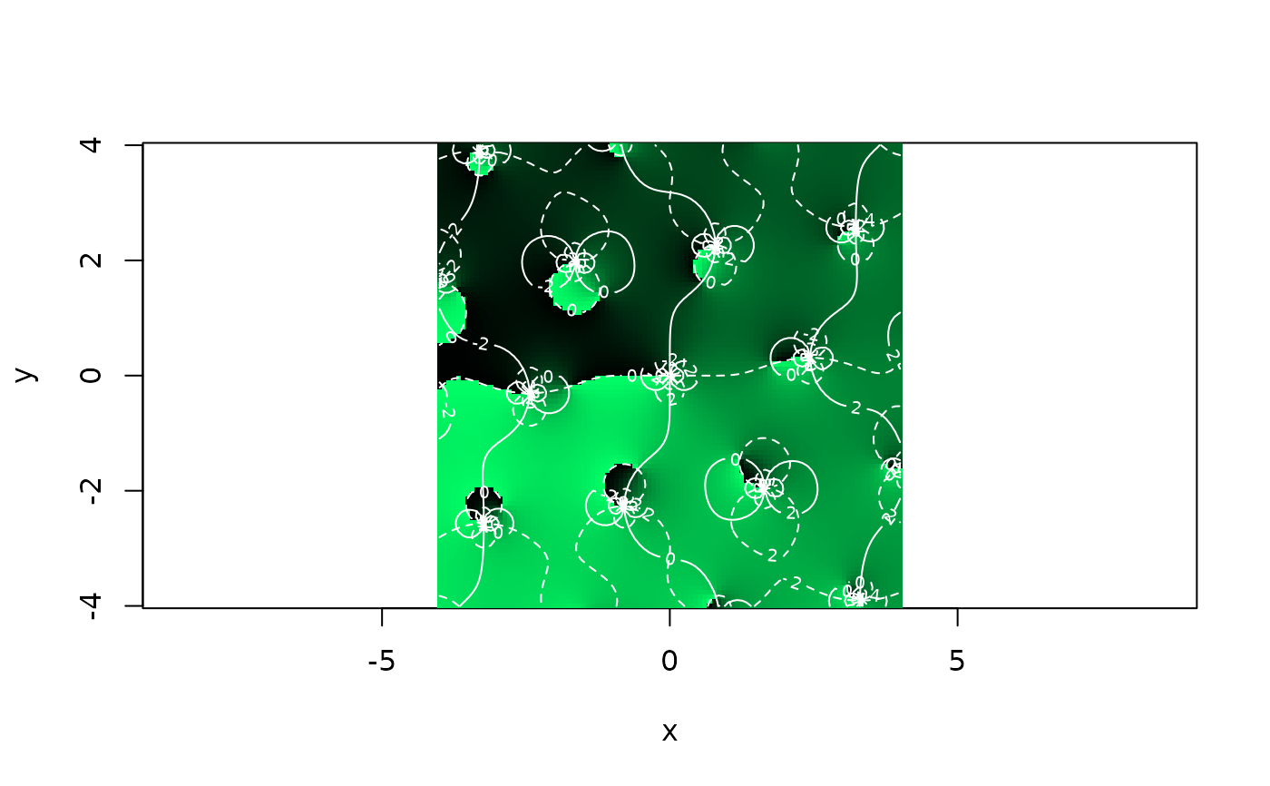
view(x,x,limit(zeta(z,c(1+1i,2-3i))),nlevels=6,scheme=4,col="white")


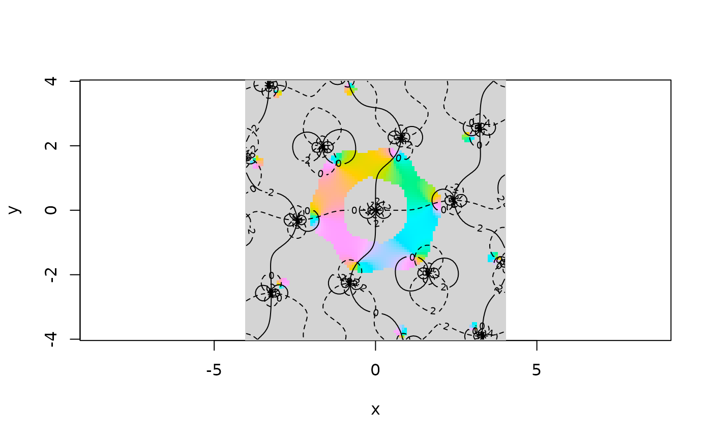
# Now an example with a bespoke colour function:

 fun <- function(z){hcl(h=360*wrap(Arg(z)),c= 100 * (Mod(z) < 1))}
 view(x,x,limit(zeta(z,c(1+1i,2-3i))),nlevels=6,scheme=fun)


view(scheme=10, show.scheme=TRUE)
#> function (z) 
#> {
#>     hsv(h = wrap(Arg(z)), v = scale(exp(-Mod(z))))
#> }
#> <bytecode: 0x560ba78233d0>
#> <environment: 0x560ba8032e50>